Characterization of Critical Camera Performance Parameters via Photon Transfer Technology

Dark and Photon Transfer Curves: what they are and what we learn from them
(Richard Crisp, www.narrowbandimaging.com, 8 February 2008)

What is a Dark Transfer Curve?
A Dark Transfer Curve is an application of the Photon Transfer analysis method pioneered by Jim Janesick and Tom Elliott of JPL for the specific task of assessing the characteristics and performance of electronic imaging systems such as CCD cameras. The tool permits empirical data to be reduced and plotted in a particular way so that critical system performance parameters can be readily extracted.

To make a DTC plot you end up plotting the following data that is measured from a camera system:

1) Total noise (Dark Shot Noise + Dark Fixed Pattern Noise + Read Noise) vs Signal
2) Dark Fixed Pattern Noise vs Signal
3) Dark Shot Noise vs Signal

The things we learn from the DTC are:

1) Camera conversion gain (e- / DN)
2) Read noise ( in DN or absolute units such as e-)
3) DSNU factor
4) Full well capacity (if you take long enough exposures)
5) And the data can permit you to calculate the dark current Quality factor (the room temperature dark current/unit-area) and doubling temperature

How to do it:
Take a collection of identical pairs of dark exposures with varying signal levels from very low (like a bias frame) to very high (near full well). You will need very accurate offset values so the best thing to do is to overscan the horizontal shift registers if a CCD is used. For a CMOS sensor you cannot take overscan data so a collection of bias frames
averaged together can give you the pixel by pixel offset values.

Data reduction:
The first thing is to determine the offset and subtract that from the raw signal. I use Excel to do that as I will be making many calculations with columns of numerical data. Then you need to measure the Standard Deviation of a region of the image. The more pixels in the sample window, the more accurate is the result. I use 100 x 100 (10,000 pixels) and that gives a statistical accuracy of (sqrt(2/#-pixels). For 10,000 pixels the accuracy is therefore in the 1.4% error range and is a convenient size to use on most sensors.

The next thing is to difference pairs of identical dark frames. This results in removal of the Dark Fixed Pattern noise and the standard deviation of this difference is equal to sqrt(2) * the remaining noise, which is Dark Shot Noise and Read noise in a quadrature sum.

Using the expression for the quadrature adding of uncorrelated noise sources, you can compute the Dark Fixed Pattern Noise for each Signal level in a separate column
Then the Total Noise, the quadrature sum of the Dark Shot Noise and Read Noise, and the Dark Fixed Pattern noise can be plotted on LOG LOG scale versus Signal. The units will be in DN (also known as ADU in the amateur astronomy community). A sample Excel Spreadsheet layout is shown below:

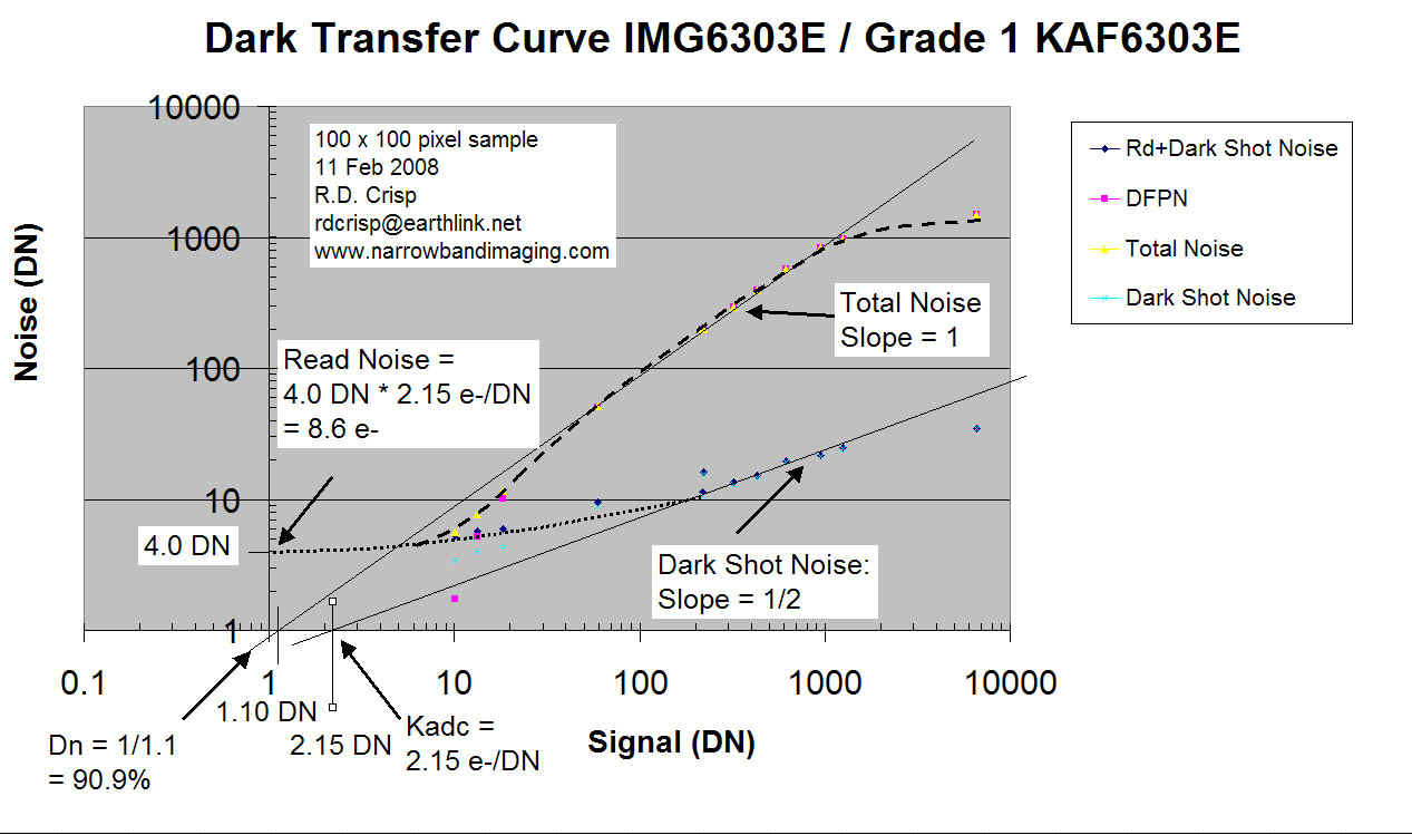
The Y intercept of the Total Noise is the Read Noise. Once the read noise is known you can again use the quadrature formula to isolate the Dark Shot Noise and that is added to the DTC plot: again plotting noise against signal. The final plot will look like this:

Interpretation
There are two major curves on the plot of interest: the Dark Shot Noise and the Dark Fixed Pattern noise. The slope of the Dark Shot noise will always be ½ when plotted on LOG LOG scale. The Slope of the Dark Fixed Pattern Noise will always be 1: again when plotted on LOG LOG scales. The DSNU is measured directly from the plot: it is the X intercept of the extrapolated Slope=1 portion of the Dark Fixed Pattern Noise curve. It is dimensionless (or expressed in percentage).

The Kadc (camera gain) is measured directly as well: it is the X intercept of the Slope = ½ portion of the Dark Shot Noise Curve. It will have dimensions of e- / DN. If the dark integrations are long enough, you can observe full well being approached as the slope of the curves will show a change on the high signal level end of the curves.

If you record the integration times and temperatures when the data is collected you can also calculate the Dark Figure of Merit (a room temperature measurement of e-/sec/pixel) or (e-/sec/cm^2) and that number can be used along with the energy gap equation to
predict the dark current at any operating temperature. The energy gap equation is more accurate than the doubling temperature method but that can give good results over a comparatively small temperature excursion from the reference temperature.

Additionally if you have dark integrations at other temperatures and exposure times you can calculate the doubling temperature as well. So there are a number of important parameters that can be learned from these plots.

Related Technology
The technique of plotting noise against signal can be also used to create Photon Transfer Curves. Instead of Dark Exposures you use light exposures. Many things can be learned from those plots including:

1) Read Noise
2) Signal Shot Noise
3) Signal Fixed Pattern Noise
4) Camera gain (Kadc)
5) Full Well
6) The effectiveness of flat fielding (are you improving the image by applying flats or not?)
7) And a host of other parameters of interest.

Photon transfer curve (taken with light on)

Using a similar approach but with the light on and taking flat fields, a Photon Transfer Curve can be created. This tool is useful for measuring camera linearity, full well capacity, camera gain, Photo Response Non-Uniformity, and various noise sources, charge skimming and so on.

The procedure is nearly identical except instead of working with Dark Frames, you take pairs of identical flat fields with varying exposure from bias frames to full well.

Sample Spreadsheet Layout:

Richard Crisp

8 February 2008

this sensor was deployed initially in early 2006. Since that time it has aged significantly due to cumulative radiation damage. to see its cosmetics and to see the impact of cooling on the cosmetics see this page:

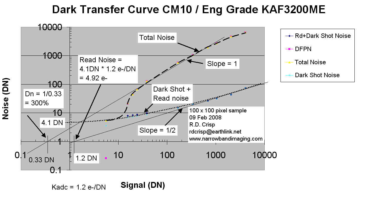
This sensor has very high noise as shown on this graph. Compare with the DTCs for the Grade 1 KAF6303 and the TK1024 to see the differences. To use the sensor effectively requires a combination of deep cooling and shorter exposures. The longer the exposure the deeper the cooling needs to be to prevent the very high DFPN from making the image noisy. Even though the DFPN can be subtracted out, the resulting images are noisier when there was significant DFPN prior to removal. By cooling more and by knowing the dark current generation rate, a cooling level can be established to make the DFPN so small as to be insignificant.

Operating it at -25C gives moderately noisy images even with 10 minute exposures.

rdcrisp@earthlink.net
www.narrowbandimaging.com